Chapter 4 Configuration

Before calculating the VIs in VICAL, a series of parameters that correspond to the configuration must be selected.

4.1 General configuration

When starting, to estimate the VI of any surface the user has two options: i) digitize polygons or ii) Use a GEE vector file. In addition, you need to configure other options, these are:

1). Date range: It is necessary to enter a start and end date, which corresponds to the interval in which you want to estimate the VIs (Figure 4.1). The date must have the following format: AAAA-MM-DD, Four digits for the year, two for the month and two for the day.

Figure 4.1: Date Range TextBox

VICAL uses this interval to search for available Landsat or sentinel-2 images, and with these images estimate VIs. VICAL by default sets the end date as the current date and the start date one year ago to the current date.

2) Cloud Percentage: A maximum cloud threshold must be entered, by default it is set to 30% (Figure 4.2).

Figure 4.2: Cloud Percentage Threshold

3). Satellite: four available options are derived from landsat and sentinel-2 satellites (described in the section 2 Satellites) (Figure 4.3):

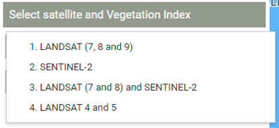
Figure 4.3: Satellites and sensors available at VICAL

 i) Landsat (7, 8 y 9): returns Landsat images from sensors 7, 8 and 9 that are within the user-defined interval and with a maximum cloud threshold. Landsat 7 ETM+ data were spectrally fitted to Landsat 8 and 9 spectral bands (OLI and OLI-2) using the procedure recommended by (Roy 2016) to generate a single set of harmonized data.

 ii) Sentinel-2: returns Sentinel-2 images that are within the user-defined interval and with the maximum cloud threshold.

 iii) Landsat (7, 8 y 9) and Sentinel-2: Returns both Landsat (7, 8 and 9) and Sentinel-2 images. Sentinel-2 MSI data are spectrally fit to Landsat-8 and 9 (OLI and OLI-2) spectral bands using the procedure recommended by (Claverie 2018). Landsat 7 ETM+ data were spectrally fitted to Landsat 8 and 9 spectral bands (OLI and OLI-2) using the procedure recommended by (Roy 2016). In this way a single set of harmonized data is generated.

 iv) Landsat (4 y 5): returns LandSat -4 and 5 images that are within the defined interval and with a maximum cloud threshold.

4). Vegetation index: The user can select from 23 VIs commonly used in agricultural applications (Figure 4.4), The formulas for each vegetation index are found in the section 3 Vegetation Indices.

Figure 4.4: Vegetation Index Selector

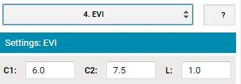
Figure 4.5: Coeficientes de IV

5) other additional functions: VICAL allows you to select additional options (Figure 4.6), for example:

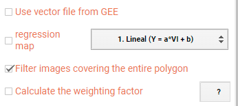
Figure 4.6: Optional configuration in VICAL

i) Use a GEE vector file: As indicated in the initial part of this chapter, the user can use a GEE vector file (polygon type). For this option, you must enter a URL address (Table ID) of the vector file that has been uploaded to GEE (Figure 4.7). in this way, even if there are digitized polygons, VICAL recognizes that the VIs must be calculated on the polygons of the vector file.

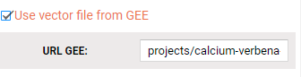
Figure 4.7: Table ID of the GEE vector file

ii) regression map: The user obtains as a result a regression map based on the values of the calculated VIs. You can select between four types of functions: linear, quadratic, potential and exponential, and then you need to enter the adjustment coefficients for the selected function (Figure 4.8).

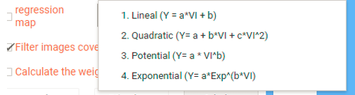
Figure 4.8: Functions considered

iii) Filter images that cover the entire polygon: Images that completely cover the polygon(s) are filtered, otherwise images are displayed even if they cover a certain percentage of the polygon. This option is useful for polygons that cover large surfaces (hundreds of hectares).
iv) Calculate weighting factor (WF): WF is the ratio of the VI value in a pixel to the average VI in the polygon (parcel). It is calculated for each digitized polygon. The WF in an agricultural parcel is a standardized indicator of the productive potential of each pixel of an image.

5) Calculate: : When the options have been configured, click on calculate and at least three layers will be shown on the map: i) RGB image of the first image found in the set interval, ii) VI map, iii) digitized polygons.

4.2 Using digitized polygons

The user can digitize any parcel (polygons) using the drawing tools found in the upper left corner of the map (Figure 4.9). VICAL recognizes that VIs must be calculated on these polygons.

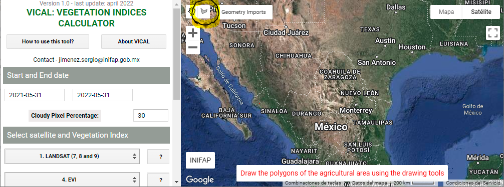
Figure 4.9: Drawing tools

This option is useful when there are few parcels where you want to estimate VIs (Figure 4.10). O bien, It is also useful when you want to download VIs for a particular area regardless of parcel boundaries. (Figure 4.11).

To edit the polygon or create a new polygon, click on the “Edit and New Polygon” buttons, respectively. These options are available after a calculation has been performed.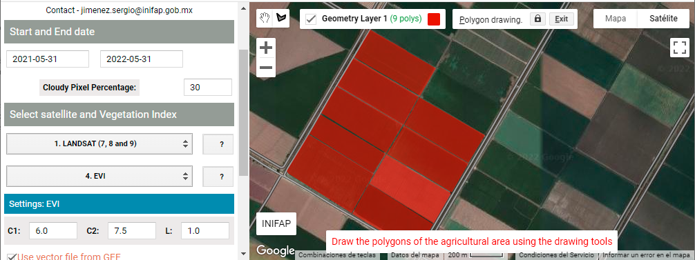

Figure 4.10: Digitized parcels

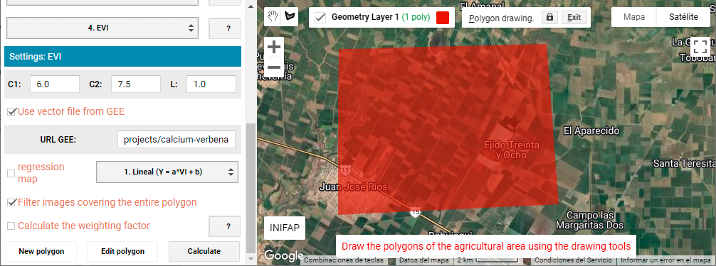
Figure 4.11: poligono digitalizados

4.3 Using GEE vector file

For this option, the user must enter the URL (Table ID) of the vector file with which the calculations are to be performed; this indicates that you must have a GEE account and import a polygon-type vector file into your account.

The *Table ID can be obtained by left clicking on the file found in the Assets** tab of your GEE account (Figure 4.12).

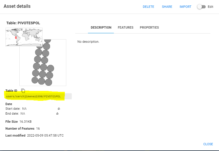
Figure 4.12: vector file details

So that the vector file can be used in VICAL, you must have the “Anyone can read” box activated (Figure 4.13).

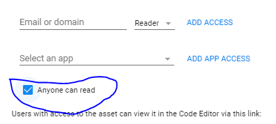
Figure 4.13: Share option view

References

Claverie, et al, Ju. 2018. The Harmonized Landsat and Sentinel-2 Surface Reflectance Data Set. Remote Sensing of Environment, 219, 145–161. https://doi.org/10.1016/J.RSE.2018.09.002.

Roy, et al, Kovalskyy. 2016. Characterization of Landsat-7 to Landsat-8 Reflective Wavelength and Normalized Difference Vegetation Index Continuity. Remote Sensing of Environment, 185, 57–70. https://doi.org/10.1016/J.RSE.2015.12.024.